Logistic map
This is not a math tutorial. See Why am I writing about math?
The logistic map is a discrete dynamical system defined by the quadratic difference equation.1
A dynamic system is a system in which a function describes the time dependence of a point in an ambient space, such as in a parametric curve.2
The logistic map function:
Where:
n: discrete time stepsx_n: the value or state at time stepnr: a constant parameter (usually between 0 and 4) that controls the system’s behavior
The equation says: “the population at the next time step equals r times the current population
times 1 minus the current population.”
What the logistic map models #
The logistic map was originally conceived as a model of population growth [source: Claude]. I’m
thinking of r as representing rate of growth, rx_n as growth, and (1 - x_n) as a limiting
factor.
Behavior for different ranges of r #
r < 1: population dies outrbetween 1-3: population stabilizes to a fixed valuerbetween 3-3.57: population oscillates between 2, then 4, then 8 values. See Periodic-doubling bifurcation . “…a periodic-doubling bifurcation occurs when a slight change in a system’s parameters causes a new periodic trajectory to emerge from an existing periodic trajectory — the new one having double the period of the original. With the doubled period it takes twice as long (or, in a discrete dynamical system, twice as many iterations) for the numerical values visited by the system to repeat themselves.”3r > 3.57: chaos, the population jumps around unpredictably, but the equation is completely deterministic. Shows how simple rules can produce complex behavior.
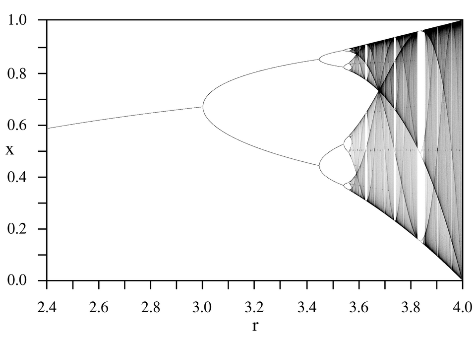
By PAR - Own work, Public Domain, https://commons.wikimedia.org/w/index.php?curid=323398
A bifurcation diagram for the Logistic map: The horizontal axis is the r parameter, the vertical axis is the x variable. The image was created by forming a 1601 x 1001 array representing increments of 0.001 in r and x. A starting value of x=0.25 was used, and the map was iterated 1000 times in order to stabilize the values of x. 100,000 x -values were then calculated for each value of r and for each x value, the corresponding (x,r) pixel in the image was incremented by one. All values in a column (corresponding to a particular value of r) were then multiplied by the number of non-zero pixels in that column, in order to even out the intensities. Values above 250,000 were set to 250,000, and then the entire image was normalized to 0-255. Finally, pixels for values of r below 3.57 were darkened to increase visibility.4
A basic Python logistic map implementation #
r = 3.5  # r = 3.5, oscillates between 4 points
x_state = 0.2


def logistic_map(x):
    return r * x * (1 - x)


# things stabilize by iteration 1000, possibly long before that
for i in range(1000):
    x_state = logistic_map(x_state)
    if i > 900:
        print(x_state)
Oscillation has stabilized to 4 states:
0.5008842103072179
0.8749972636024641
0.38281968301732416
0.8269407065914387
0.5008842103072179
0.8749972636024641
0.38281968301732416
0.8269407065914387
Attempting to get an 8-period orbit. It’s close:
r = 3.564  # r = 3.564, oscillates between approximately 8 points
x_state = 0.2


def logistic_map(x):
    return r * x * (1 - x)


# things stabilize by iteration 1000, possibly long before that
for i in range(10000):
    x_state = logistic_map(x_state)
    if i > 9000:
        print(f"{i % 8}: {x_state}")
Output:
0: 0.490948165280856
1: 0.8907079811232064
2: 0.34694568270634296
3: 0.8075110759135015
4: 0.553977247711016
5: 0.8806161317840935
6: 0.37468816784444325
7: 0.8350343109885577
0: 0.49094816528094537
1: 0.8907079811232124
2: 0.34694568270632625
3: 0.8075110759134831
4: 0.553977247711056
5: 0.880616131784078
6: 0.3746881678444851
7: 0.8350343109885952
Feigenbaum constants #
The term bifurcation is used to describe the points where the system’s behavior changes qualitatively, e.g., splitting from a period-1 orbit to a period-2 orbit, to a period-3 orbit…
- Period-1 → Period-2 (bifurcates at r₁ ≈ 3.0)
- Period-2 → Period-4 (bifurcates at r₂ ≈ 3.449)
- Period-4 → Period-8 (bifurcates at r₃ ≈ 3.544)
- Period-8 → Period-16 (bifurcates at r₄ ≈ 3.564)
Feigenbaum discovered that the spacing between consecutive bifurcation points shrinks by a constant ratio: .
This means:
Each bifurcation happens about 4.669 sooner than the previous one. This holds true for any system that undergoes period doubling routes to chaos.
-
Wikipedia contributors, “Logistic map,” Wikipedia, The Free Encyclopedia, https://en.wikipedia.org/w/index.php?title=Logistic_map&oldid=1320815055 (accessed December 8, 2025). ↩︎
-
Wikipedia contributors, “Dynamical system,” Wikipedia, The Free Encyclopedia, https://en.wikipedia.org/w/index.php?title=Dynamical_system&oldid=1316886564 (accessed December 8, 2025). ↩︎
-
Wikipedia contributors, “Period-doubling bifurcation,” Wikipedia, The Free Encyclopedia, https://en.wikipedia.org/w/index.php?title=Period-doubling_bifurcation&oldid=1315027005 (accessed December 8, 2025). ↩︎
-
Wikimedia Commons contributors, “File:LogisticMap BifurcationDiagram.png,” Wikimedia Commons, https://commons.wikimedia.org/w/index.php?title=File:LogisticMap_BifurcationDiagram.png&oldid=452366429 (accessed December 8, 2025). ↩︎