Embeddings visualization with UMAP

This is not a math tutorial. See Why am I writing about math?

Uniform Manifold Approximation and Projection (UMAP) is a dimension reduction technique that can be used for visualization similarly to t-SNE, but also for general non-linear dimension reduction. The algorithm is founded on three assumptions about the data

1. The data is uniformly distributed on [a] Riemannian manifold;
2. The Riemannian metric is locally constant (or can be approximated as such);
3. The manifold is locally connected.

From these assumptions…¹

From those assumptions I realize I’m in over my head. Backtracking a bit…

This gets clearer (in a non-mathematical way) further down in: An attempt at clarifying UMAP’s assumptions.

What is Euclidean space?

“Euclidean space is the fundamental space of geometry, intended to represent physical space. Originally, in Euclid’s Elements, it was the three-dimensional space of Euclidean geometry, but in modern mathematics there are Euclidean spaces of any positive integer dimension n, which are called Euclidean n-spaces….”²

Examples:

• $\mathbb{R}^1$ (Real line): the number line
• $\mathbb{R}^2$ (Euclidean plane): a flat sheet of paper or graph
• $\mathbb{R}^3$ (Euclidean 3D space): (a representation of) familiar 3D space

For details about typing math symbols in markdown files, see notes / Typing math symbols with LaTeX.

“Euclidean space is the fundamental, ‘flat,’ multi-dimensional space of classical geometry where standard rules apply, allowing us to measure distances and angles with the familiar Pythagorean theorem…”³

What is a manifold?

“In mathematics, a manifold is a topological space that locally resembles Euclidean space near each point. More precisely, an n-dimensional manifold, or n-manifold…is a topological space with the property that each point has a neighborhood that is homeomorphic to an open subset of n-dimensional Euclidean space.”⁴

What is a space in the context of math?

A space is a set of points.

What is a topological space?

• a geometrical space where closeness is defined but can’t necessarily be measured by a numeric distance.
• a set of points, along with an additional structure called a topology

A topology is a set of neighbourhoods (for each point in a space(?)) that allows some concept of “closeness” to be defined.(?)

What is a neighbourhood?

“…a neighbourhood of a point is a set of points containing that point where one can move some amount in any direction away from that point without leaving the set.”⁵

In the image below: a set $V$ in the plane is a neighbourhood of a point $p$ if a small disc around $p$ is contained in $V$. The small disc around $p$ is an open set $U$.⁶

What is a Riemannian manifold?

I’ll start with “[a]ny smooth surface in three-dimensional Euclidean space is a Riemannian manifold with a Riemannian metric coming from the way it sits inside the ambient space.”⁷

The ambient space of a line is the line of real numbers, the ambient space of a point in 2D space is Euclidean 2D space?

A Riemannian manifold is a space that locally resembles Euclidean space.⁸ Remember that a manifold is a topological space that locally resembles Euclidean space.

What is a Riemannian metric?

A Riemannian manifold has a Riemannian metric — a way to measure lengths, angles, (and volumes(?)) across the space. Getting back to the task at hand (understanding UMAP (uniform manifold approximation and projection)), a space being a Riemannian manifold implies that it’s meaningful to talk about distances between points — distances between vector embeddings.

The second assumption about the data that’s made by UMAP is “the Riemannian metric is locally consistent (or can be approximated as such).”⁹

An attempt at clarifying UMAP’s assumptions

A manifold is a shape that locally looks flat, even if it’s curved globally. (The earth is a sphere by locally we treat it as flat.)

There’s a hypothesis in ML (the “manifold hypothesis” ) that high dimensional data like language actually lives on a lower dimensional manifold.

That means that this site’s 384 dimensional embeddings aren’t spread uniformly across all the dimensions. They live (mostly(?)) on a lower-dimensional surface (a manifold). That’s why UMAP can compress them down to 2D without losing too much information.

An explanation (simplification) of UMAP’s assumptions:

• “Uniformly distributed on a Riemannian manifold”: the datapoints are spread evenly across the manifold. “Riemannian” means that it’s a smooth(?) manifold, where you can measure distances and angles (it has a Riemannian metric).
• “Riemannian metric is locally constant”: the way that distances is measure is consistent within small neighborhoods. A possible analogy, small distances on the earth can be measured with a ruler. To measure something like half-way around the earth, you’d need to tool that accounted for the earth’s curvature.
• “Manifold is locally conected”: there are no sudden jumps or tears. I’m not sure what a sudden jump or tear would “look” like.

UMAP is assuming the embeddings live on a smooth, lower-dimensional shape that can be flattened to 2D whild preserving the neighborhood structure.

Visualizing this site’s vector embeddings

Things are getting too abstract. I need something to hold on to.

This site’s search functionality uses a Chroma database. The process of generating the database’s embedding vectors isn’t yet fully documented (todo: document how embeddings are generated.)

Here’s an overview of the database:

import chromadb

chroma_client = chromadb.PersistentClient()
collection = chroma_client.get_collection(name="zalgorithm")

results = collection.get(include=["embeddings", "metadatas", "documents"])

print(results.keys())
# dict_keys(['ids', 'embeddings', 'documents', 'uris', 'included', 'data', 'metadatas'])

print(len(results["metadatas"]))
# 918
print(results["metadatas"][0].keys())
# dict_keys(['db_id', 'page_title', 'section_heading', 'updated_at'])

print(len(results["embeddings"]))
# 918
print(len(results["embeddings"][0]))
# 384

print(results["metadatas"][0]["section_heading"])
# SimCSE: Simple Constrative Learning of Sentence Embeddings (paper)
print(results["embeddings"][0][:10])
# [-0.00372653 -0.05460251  0.03505962  0.04954087  0.06700463  0.07712093
#   0.02034441  0.05408454  0.05195715 -0.01918259]

print(results["metadatas"][1]["section_heading"])
# The Meaning of Meaning (book)
print(results["embeddings"][1][:10])
# [ 0.00272638  0.09517232 -0.05058211  0.04337437 -0.01964302  0.00047342
#   0.04571834  0.08724379  0.04383722  0.03747305]

So there are (currently) 918 entries in the database. Each entry has an id, embedding, metadata, and more.

The embeddings are 384 dimension vectors. (Generated with Chroma DB’s default embedding model, the all-miniLM-L6-v2 model from the Sentence Transformers library.)

Embedding metadata is data that I’ve added to the database. For example, the metadata "db_id" key ("results["metadatas"][<row_number>]["db_id"]) makes it possible to get an embedding’s associated HTML fragment from an SQLite database.

The HTML headings associated with each embedding are in the metadata "section_heading" field. A quick glance shows that the embedding associated with the heading “SimCSE: Simple Constrative Learning of Sentence Embeddings (paper) " is different from the embedding associated with the heading “The Meaning of Meaning (book)”. This is as expected.

Installing lmcinnes/umap

It’s got a few dependencies: https://github.com/lmcinnes/umap:

Python 3.6 or greater

• numpy
• scipy
• scikit-learn
• numba
• tqdm
• pynndescent

PyNNDescent

PyNNDescent is a Python nearest neighbor descent for approximate nearest neighbors. It provides a python implementation of Nearest Neighbor Descent for k-neighbor-graph construction and approximate nearest neighbor search…¹⁰

GitHub: https://github.com/lmcinnes/pynndescent

First visualization attempt

Just getting something to appear:

import chromadb
import numpy as np
import matplotlib.pyplot as plt
import umap
import random

chroma_client = chromadb.PersistentClient()
collection = chroma_client.get_collection(name="zalgorithm")

results = collection.get(include=["embeddings", "metadatas", "documents"])

embeddings = np.array(results["embeddings"])
metadatas = results["metadatas"]

reducer = umap.UMAP(n_neighbors=15, min_dist=0.1, metric="cosine")

embedding_2d = reducer.fit_transform(embeddings)

plt.scatter(embedding_2d[:, 0], embedding_2d[:, 1], s=140, alpha=0.75)

for i, metadata in enumerate(metadatas):
    print(f"{i}: {metadata['page_title']}: {metadata['section_heading']}")
    label = str(i)
    x = embedding_2d[i, 0]
    y = embedding_2d[i, 1]
    plt.text(x, y, label, ha="center", va="center", color="white", fontsize=6)

plt.show()

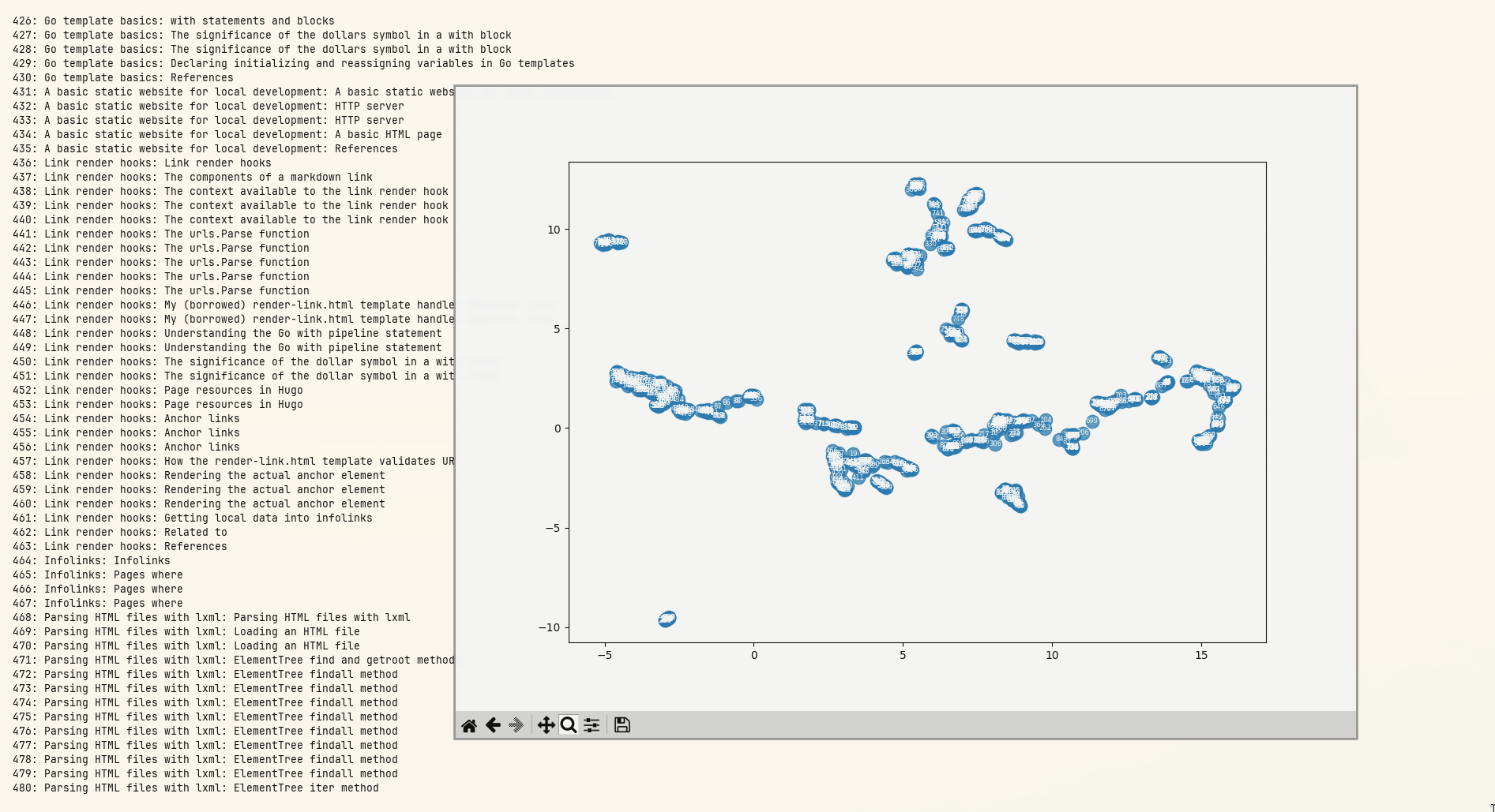
At that zoom level an overall pattern can be seen, but the results are illegible. Fortunately, PyPlot windows can be zoomed in on:

From there I can see:

• 833 (farthest left): Roger Bacon overview: The three dignities
• 327 (hidden behind 833): Scientia Experimentalis: Scientia Experimentalis (also Roger Bacon related)
• 834 (to the right of the previous two): Roger Bacon overview: The three dignities
• entries 6, 8, 10, 12 (the highest cluster to the left): all related to alchemy in the middle ages
• 17 (slightly to the left of the previous cluster): Natural Philosophy: Natural Philosophy

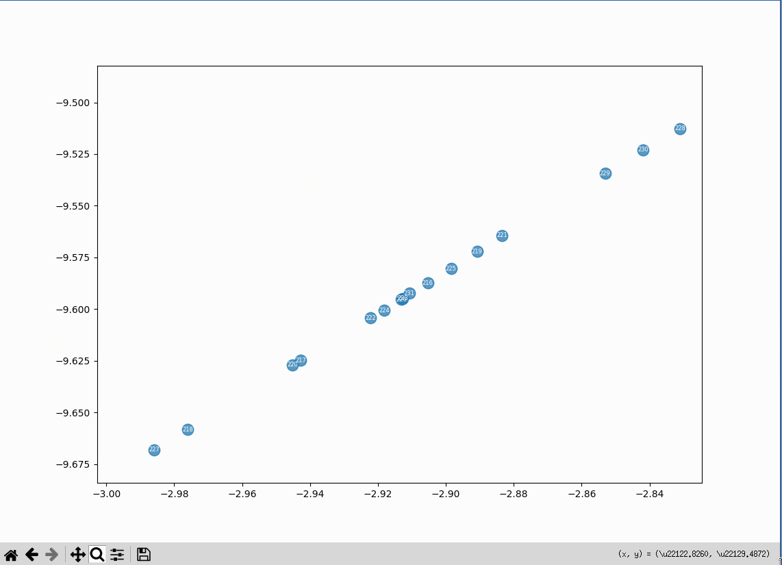
The three entries at the bottom right of the plot:

• 28: Roger Bacon as Magician: What optical devices did Bacon have?
• 29: Roger Bacon as Magician: What is a broken mirror in this context?
• 30: Roger Bacon as Magician: Who are the “jugglers” that are mentioned by Molland?

There’s a definite order to the results. My guess is that section headings are having a strong effect on the vectors. The text that’s used to generate the vectors has the full heading path of each section prepended to it, so there’s some heading context that’s not being shown in this (loose) analysis of the data.

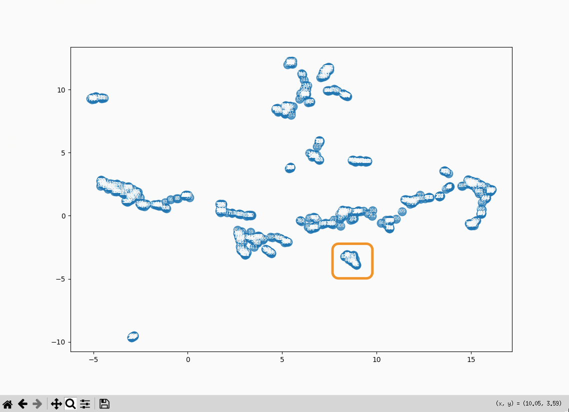
What’s in the cluster that’s closest to the center?

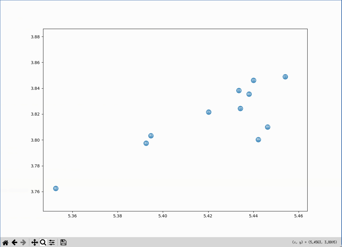
A bunch of embeddings related to the cp command. There aren’t a lot of posts like that on the site:

• 375: Copy a directory and its contents from the command line: Copy a directory and its contents from the command line
• 376: Copy a directory and its contents from the command line: Copy a directory and its contents from the command line
• 377: Copy a directory and its contents from the command line: The cp command can create the destination directory
• 378: Copy a directory and its contents from the command line: Attempting to copy a directory with cp without setting options
• 379: Copy a directory and its contents from the command line: Copy only the
• 380: Copy a directory and its contents from the command line: What are file attributes?
• 381: Copy a directory and its contents from the command line: What does the no-dereference flag do?
• 382: Copy a directory and its contents from the command line: What does the no-dereference flag do?
• 383: Copy a directory and its contents from the command line: What does the preserve=links flag in combination with the no-dereference flag do?
• 384: Copy a directory and its contents from the command line: References
• 386: Retrieval practice scratchpad: The cp command

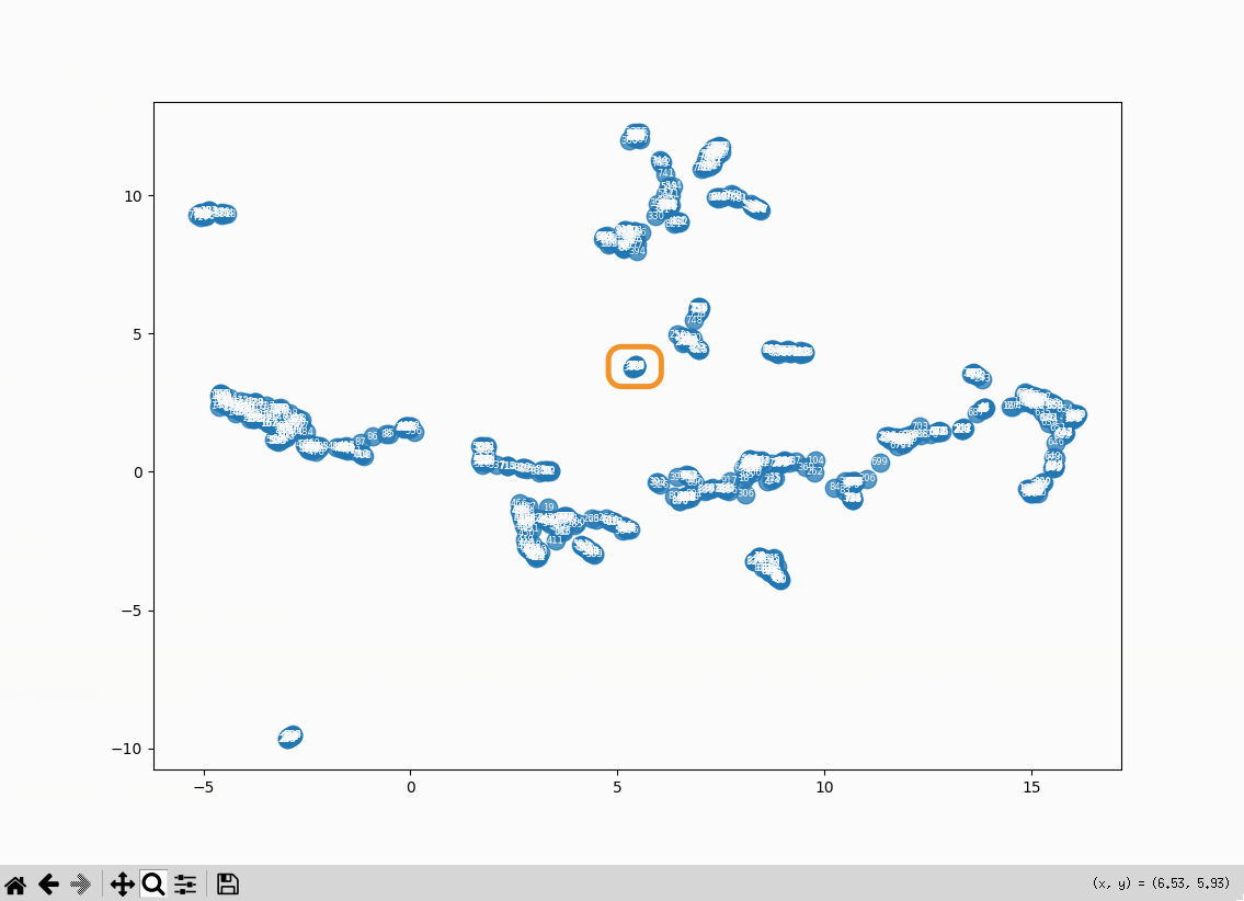
Vectors (remember these are 2D representations of vectors) in the far left, y ~= 0 part of the plot are all related to XML.

Vectors in the far right y ~= 0 are all related to Newton’s method.

Just to the left of the Newton’s method vectors are vectors related to Halley’s method.

The cluster at the far bottom left of the plot is made up of embeddings related to an issue with video rendering on the Omarchy Linux distribution. They form an oddly straight line:

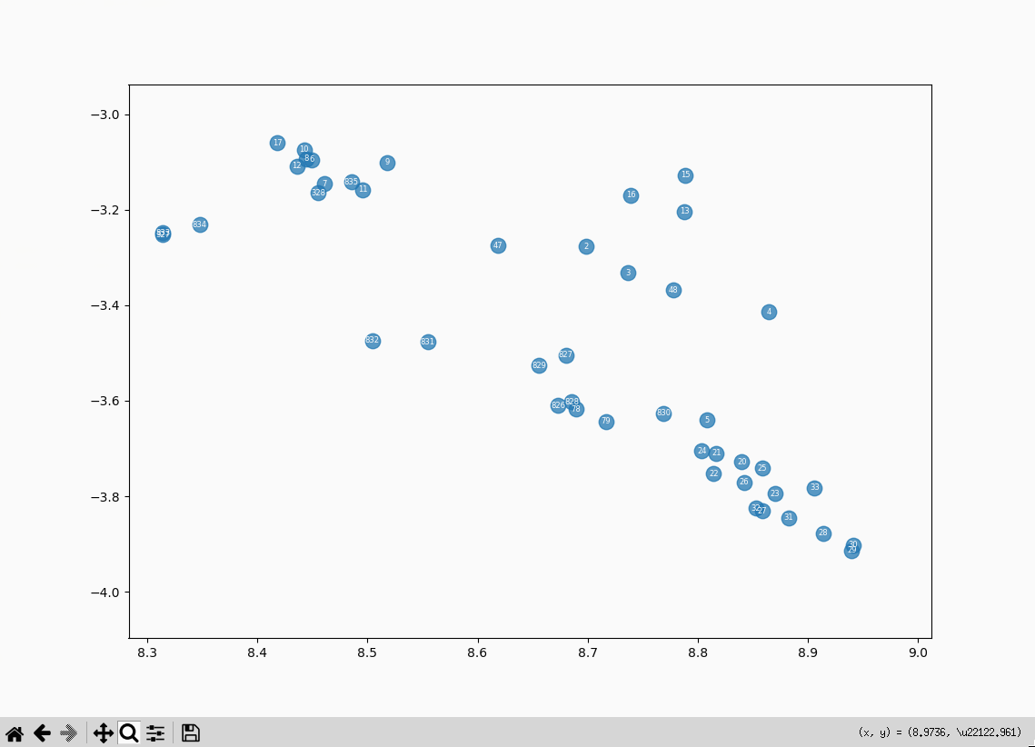
Literary Machines cluster

Maybe the tightest cluster in the plot is made of embeddings related to the book Literary Machines. The embeddings are mostly quotes from the book:

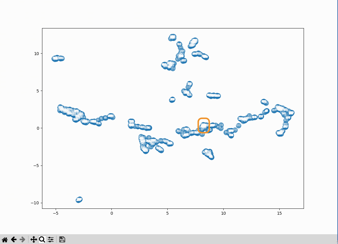
Using vector embeddings to reveal the structure of a group of documents

What’s interesting about the Literary Machines cluster is that Ted Nelson is writing about ways presenting the structure of information to the reader. Possibly something along those lines can be done with vector embeddings.

References

McInnes, Leland. “UMAP: Uniform Manifold Approximation and Projection for Dimension Reduction.” https://umap-learn.readthedocs.io/en/latest/ .

Wikipedia contributors. “Euclidean space.” Accessed: January 14, 2026. https://en.wikipedia.org/wiki/Euclidean_space .

Wikipedia contributors. “Manifold.” Accessed: January 14, 2026. https://en.wikipedia.org/wiki/Manifold .

Wikipedia contributors. “Neighbourhood (mathematics).” Accessed: January 14, 2026. https://en.wikipedia.org/wiki/Neighbourhood_(mathematics) .

Wikipedia contributors. “Riemannian manifold.” Accessed: January 14, 2026. https://en.wikipedia.org/wiki/Riemannian_manifold .